
Most transport operators know their business is seasonal. They don’t always plan as if it is. There’s a gap between the intuition “we get busier in summer” and the operational discipline of actually building a calendar, a fleet allocation strategy, a staffing rhythm, and a maintenance schedule around the shape of the annual demand curve. That gap is where money quietly leaks. Bikes are parked when they should be ridden. Drivers are scheduled when there’s no demand for them. Maintenance happens during peak season when it should have happened in the trough.
Transport seasonality is the structural reality that demand for any movement based business, bike share, ride share, public transit, last-mile delivery, courier networks, regional logistics, that varies predictably across the year. Not week to week, which is volatile and hard to forecast, but month to month, which is broadly knowable years in advance. The seasonal shape doesn’t change much from year to year. What changes is whether the operator builds the calendar around it or pretends it doesn’t exist.
This article is about that calendar. Specifically, what transport seasonality actually looks like when you measure it properly, what operational decisions it should change, and why the shoulder seasons (the months between peak and trough) are usually the hardest to plan for. The argument here is grounded in a year of bike share data from a real urban network, but the principles apply to any transport or mobility business with a meaningful weather or behavioural dependence.
What the Seasonal Curve Actually Looks Like
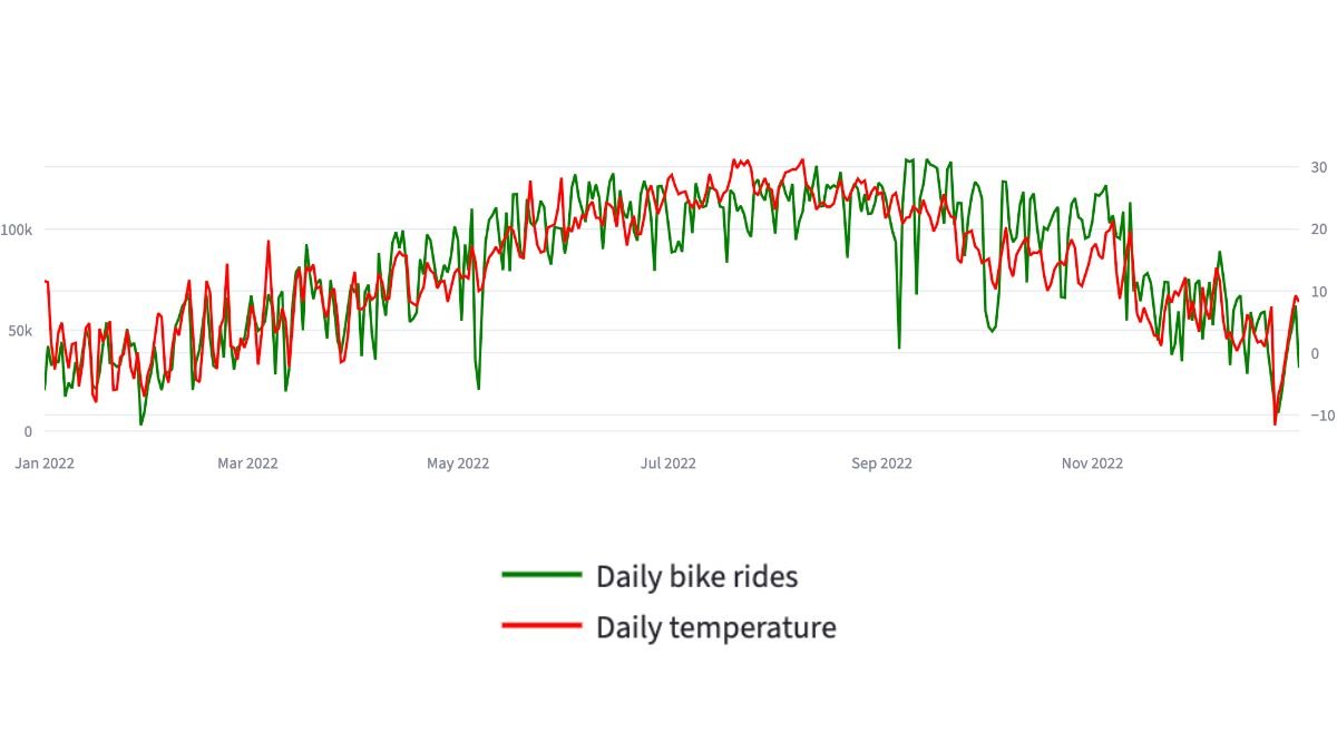
The Citi Bike 2022 public dataset gives an unusually clean picture of transport seasonality at scale. Across nearly 30 million trips in a single year, the monthly distribution was unambiguous. August was the peak month at 3,565,961 trips. September followed at 3,404,153. July at 3,388,479. June at 3,337,836. The summer months together carried roughly 47% of all annual trip volume.
Winter was the inverse. January, the lowest month, recorded 1,014,916 trips, roughly 3.5 times less than August. February (1,195,117) and December (1,587,127) rounded out the winter trough. The shape of transport seasonality isn’t a gentle wave; it’s a sharp asymmetric curve with a long ramp up through spring, a four month peak, and a steep drop through autumn into winter.
The contrast at the daily level made the seasonality issue concrete. The busiest single day in the dataset was 14 September 2022 with 134,851 trips and an average temperature of 22.9°C. The quietest day was 29 January 2022 with 2,809 trips and an average temperature of -4.8°C. That’s roughly a 48-fold swing in daily demand between the warmest and coldest days of the same year, in the same city, in the same network.
This is what transport seasonality looks like when you measure it properly. It’s not a footnote on a quarterly report. It’s the dominant variable shaping daily, weekly, and monthly operational reality. And the Citi Bike case study walks through the full year of demand data in more detail, the seasonal curve sits at the centre of every operational recommendation in that project.
The same shape, peak summer, trough winter, sharp asymmetric curve, shows up in other outdoor dependent transport businesses. Bike share is the cleanest example of transport seasonality because it’s the most weather exposed, but ride share, regional transit, and delivery networks all show seasonal patterns of varying intensity. The structural lesson holds: if the curve exists, plan around it.
How Seasonality Reshapes the Operational Calendar
The operational implications of transport seasonality fall into four practical buckets, and each one represents a decision that gets made differently, better when transport seasonality is built into the planning process rather than treated as a footnote.
Fleet sizing and allocation. A bike-share network running its full peak-season fleet in February is paying for inventory it doesn’t need. The Citi Bike data suggests a roughly 30–40% reduction in deployed fleet between November and April is reasonable, while still protecting supply at the highest-demand stations. That’s not a guess, it’s a number that falls out of the actual demand distribution. The same principle applies to any transport business with elastic fleet sizing: scale down during the trough months rather than spreading the full-year fleet across all twelve months equally.
Maintenance scheduling. The cheapest time to take a vehicle, a bike, or a piece of infrastructure offline for maintenance is when demand is lowest. The most expensive time is during peak. Operators who don’t build maintenance into the seasonal calendar end up doing reactive maintenance during August, when every unit out of service has a measurable revenue impact, instead of planned maintenance during January, when the marginal cost of downtime is small.
Staffing rhythm. Seasonal demand requires seasonal staffing, but the shape matters. Peak-season staffing should anticipate the summer concentration. Winter staffing should focus on maintenance, planning, and operational improvements that the peak season made impossible. Most transport businesses understaff for peak and overstaff for trough, which is exactly backwards.
Marketing and partnership timing. Sponsorship deals, advertising campaigns, partnership launches, these are easier to land and more valuable to operate during the high-attention months. A new station unveiling in February is invisible. The same unveiling in May, just before peak season, lands. Transport seasonality is a marketing calendar too, not just an operational one.
Weather is the strongest demand variable most transport operators underestimate, and seasonality is the structural way weather shows up across the year. Treating the two together, daily weather variance plus monthly seasonal shape, is what an actual operational planning framework looks like.

Why Shoulder Seasons Are the Hardest to Plan For
The summer peak and winter trough are easy to plan for in principle, because the demand levels are stable and predictable across those months. The hard part of transport seasonality is managing the shoulder seasons, March through May on the way up, October through November on the way down, where the seasonal curve is steepest. These are the months where demand changes fastest week-over-week and where operational decisions have to be most adaptive.
In March, demand can double from one week to the next as the first warm days arrive. A fleet still sized for February will be visibly under-supplied. A fleet pre-emptively sized for May will be expensive and underutilised. The operator has to read the weather forecast as a forward-looking operational signal, not a background variable, and adjust deployment in near-real-time.
The autumn shoulder is even trickier because demand falls unevenly. A warm October Saturday can produce summer-level trip volumes. The following Tuesday can drop to spring levels. Operators who scale down too fast lose revenue. Operators who scale down too slowly carry inventory cost they don’t need.
The practical answer is that shoulder seasons need their own operational rhythm, closer to weekly adjustment cycles than monthly, with weather forecasts treated as forward-looking inputs rather than reporting metrics. This is a different operating posture from peak season (steady high-demand staffing) and trough season (steady low-demand staffing). It’s the most operationally demanding phase of the year, and the one most likely to be handled by intuition rather than data.
Allocation is a separate problem from forecasting, I wrote about why fleet shortages usually show up in customer experience before they show up in the data and what to look at instead.

The Annual Planning Conversation Most Operators Skip
Most transport businesses run quarterly planning cycles. The problem is that quarters don’t match the seasonal shape. Q1 (Jan–Mar) contains both the deepest trough and the start of the spring ramp. Q2 (Apr–Jun) contains shoulder ramp and the start of peak. Q3 (Jul–Sep) is essentially all peak. Q4 (Oct–Dec) contains shoulder decline and the start of the trough.
Planning by quarter means making operational decisions inside time windows that mix radically different demand environments. The early-Q1 decisions need to be different from late-Q1 decisions. The same is true at every transition. Quarterly cadence is a finance artefact, not an operational one, and using it as the primary planning rhythm makes seasonality harder to manage rather than easier.
A better cadence for transport seasonality is two month planning cycles anchored to the seasonal shape itself: deep trough (Dec–Feb), spring shoulder (Mar–Apr), early peak (May–Jun), late peak (Jul–Sep), and autumn shoulder (Oct–Nov). Each phase is its own transport seasonality window with its own operational rhythm. Five phases, each with its own operational posture, fleet target, staffing pattern, and review rhythm. This isn’t a complicated framework. It just requires the operator to look at the actual demand shape and plan accordingly. Seasonality sets the annual rhythm, but the hourly view is where the daily operational decisions actually live. I’ve written separately about why hourly demand patterns matter for transport operators.
NOAA’s climate data is freely available for any operator to merge with their own demand records.
For operators wanting to actually do this themselves, the weather data integration guide walks through the practical steps.
What Transport Seasonality Looks Like in a Dashboard
For an operator working with the kind of demand data Citi Bike publishes, or any equivalent fleet, route, or trip data, building seasonality into the dashboard layer is what makes the framework actionable rather than theoretical. The seasonal view needs three things at minimum: monthly trip totals (the curve), monthly trip totals year-over-year (the trajectory), and average daily demand by month with weather overlaid (the variance inside the curve).
Geospatial analysis adds another dimension to the same planning conversation, because seasonality doesn’t affect every station equally. Some stations have stable year-round demand. Others swing wildly. A network-level seasonal curve hides station-level variation that the geospatial layer surfaces. Both are needed.
The closing piece is the recommendations layer, the place where the dashboard translates “here’s the seasonal shape” into “here’s what to do about it.” That layer is the difference between a reporting tool and an operational tool. It’s also the part most transport businesses are missing, because their current reports tell them what happened last month rather than what to do next month.
If a transport or mobility business is trying to build that kind of strategic operational dashboard built around the annual rhythm, that’s the work I do. And if a custom dashboard isn’t quite what you need, maybe data cleaning, ad-hoc analysis, or ongoing reporting support is the better fit, those are other data services I offer.
The seasonal curve is the most predictable thing in a transport business. The fact that most operators don’t plan around it isn’t a data problem. It’s an operational discipline problem. The data is there. The framework is straightforward. The hard part is building the calendar and sticking to it.
I build custom operational dashboards for businesses with hidden demand patterns, multi-location retail, transport and logistics, booking-based services, e-commerce, and hospitality. The work starts with the decisions you need to make, not the charts.
See how the dashboard service works → or explore other data services if you’re not sure what you need.
Pingback: Weather Data Integration: A Smart Practical Guide
Pingback: Citi Bike Case Study: A Powerful Mobility Dashboard Build
Pingback: Weather and Demand: Why Reports Miss the Biggest Variable